In the full image stylization process, areas with high-frequency texture will be approximated by stipples, whereas areas with lower-frequency texture will be approximated by closed shapes. To create the closed shapes and decide how the image is to be divided into regions, each containing pixels with similar properties, I need an image segmentation algorithm.

For now, I have chosen Simple Linear Iterative Clustering (SLIC) [1] as the segmentation algorithm. SLIC is efficient and produces regions which adhere well to edges in the image. Moreover, it is not overly difficult to implement.

SLIC demonstration

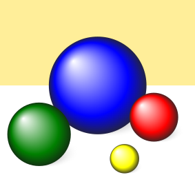
The source image, shown below, is from the Qt SVG viewer example.

Varying the "m" parameter

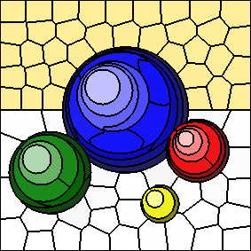
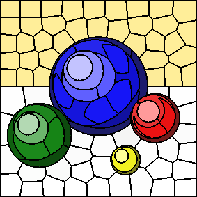
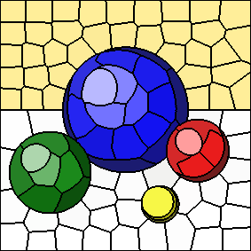
As the value of "m" increases, spatial distances to cluster centers are given more weight and colour distances to cluster centers are given less weight.

The following series of images shows the results for "m" equal to 5, 10, 20, and 40, respectively (left to right). In all cases, the number of clusters is fixed at 100. Increasing the value of "m" results in more compactly-shaped (rounder) superpixels.

Post-Processing Routine

The original description of SLIC [1] only touches on the process which follows K-Means iteration. The post-processing routine must reduce the number of connected components for each cluster to one, by merging unwanted connected components with their neighbours as appropriate. (A connected component is a set of pixels, with the property that it is possible to navigate from one pixel to any of the others without passing over pixels associated with other clusters.)

Initially, I had interpreted the description to mean the following:

• Identify connected components that lie underneath the center of their respective K-Means cluster.
• Iterate over the pixels in all other connected components and assign them to the closest connected components that were identified in the previous step. For each pixel, find the closest connected component using an algorithm such as breadth-first search, which determines shortest paths. To run breadth-first search, treat the image as a graph where each pixel is a node and there is an edge between each pixel and each of its four nearest neighbours.

The results of the above post-processing method, with an "m" value of 10, and 100 cluster centers, is shown below. It produces considerable warping of shapes in this image, because there are many crescent-shaped connected components which do not lie underneath their corresponding K-Means cluster centers.

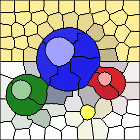
The results shown earlier use a different post-processing routine, in which the largest connected component is selected for each K-Means cluster, rather than any connected component which contains the cluster center. With this method, I still use the same process for merging the pixels of unwanted connected components into the selected connected components (i.e. breadth-first search). This post-processing routine is similar to the one suggested by Dr. Mould, except that his version assigns unwanted connected components to their largest neighbours, thus avoiding making per-pixel reassignment decisions.

For comparison, the following image depicts the raw K-Means iteration result, prior to post-processing (again, with 100 cluster centers and an "m" value of 10):

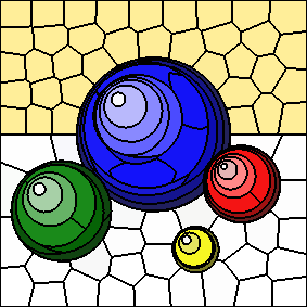
In this case, the highlights of the spheres are part of the same clusters as areas of the background. Having multiple connected components for a given superpixel makes it more difficult to use the superpixel as the input to other algorithms. Furthermore, most of the additional connected components tend to be small, and therefore serve as poor image regions.

References

1. R. Achanta et. al. "SLIC superpixels compared to state-of-the-art superpixel methods."
   IEEE Transactions on Pattern Analysis and Machine Intelligence, vol. 34,
   no. 11, pp. 2274-2281, Nov. 2012. (Authors' website for SLIC: http://ivrg.epfl.ch/research/superpixels)