Graphics, Imaging, and Games Lab

Introduction

Recolouring an image by averaging the image with a solid colour, as shown in my last two posts (http://gigl.scs.carleton.ca/node/538 and http://gigl.scs.carleton.ca/node/539), is a simple way to add contrast and visual interest to an image, provided that the average is not uniformly weighted across the image. I experimented with recolouration as kind of an end in itself, but also with the intention of predicting the results of a more general process, image retexturing.

I will use the term "retexturing" to refer to adding two images together (a source image and a texture image) to produce an image which retains patterns from both of the original images. Recolouration is simply a type of retexturing in which the texture image has no colour variation.

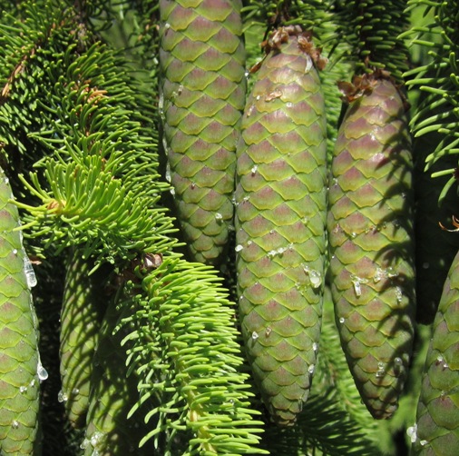
Source image for the results in this post

Method

The specific procedure that I used for retexturing is as follows:

1. Obtain a weighting image in some fashion. In this post, I used weighted images produced using three different methods. In some cases, I produced the actual weighting images by applying MATLAB's morphological erosion or dilation functions to images produced using the three methods:

   1. All values in the weighting image are 0.5, which will result in equal weighting of both the source and texture images at all pixel locations.

   2. The weighting image is derived from the residual, which is the subtraction of the smoothed image resulting from cumulative range geodesic filtering from the source image. The weighting image is obtained from the magnitude (lengths of colour vectors in RGB space) of the compressed residual. The compressed residual is obtained by the following transformation: If x is a colour channel value in the residual, then the compressed value of x is log2(x), 0, or -log2(-x) if x > 1, |x| < 1, or x < -1, respectively.

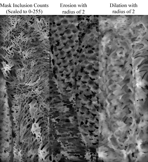
   3. The weighting image is obtained by creating a filtering mask for each pixel in the source image using cumulative range geodesic filtering, and counting the number of times that each pixel is included in any of the filtering masks. (The value assigned to a pixel in the weighting image is its count of mask inclusions.)

All weighting images were scaled to ranges of values between 0 and 1, following morphological erosion or dilation, if applicable, except that, in the last section of this post, weighting images were scaled to ranges of 0 to 0.5 or 0.5 to 1 (for reasons discussed later). If I used morphological erosion or dilation, I scaled the eroded or dilated images using the same scaling factors as for the undilated or uneroded image. Otherwise, the average increase or decrease of weighting values due to erosion or dilation would be lost by re-scaling to the full range of 0-1.

For morphological erosion and dilation, I used approximately circular, flat structuring elements without approximate decomposition (i.e. by calling strel('disk', radius, 0) in MATLAB). I achieved different levels of erosion and dilation by varying the radii (measured in pixels) of the structuring elements.

2. Obtain a texture image. I used two different texture images in this post: one composed of randomly-coloured checkers, and another produced by finding the count of mask inclusions for each pixel in the source image, which is the third method described in Step 1 above.

3. Produce the output image. I calculated the pixel values in the output image by either of the following methods, depending on whether I wanted to preferentially retexture outlier pixels (pixels with low mask inclusion counts or high residual values) or non-outlier pixels:

For all results shown in this post, I preferentially retextured non-outlier pixels, except in the last section, where noted. My intention was to apply new textures to the less visually-interesting areas of the source image, while leaving the more visually-interesting areas of the source image unchanged.

When retexturing using a random checker pattern, I averaged all pixel channel values in RGB space. In contrast, when I used counts of mask inclusions as the new texture, I converted the source image to the CIE L*a*b* colour space and averaged only its L* channel with the counts of mask inclusions.

All cumulative range geodesic filtering was conducted with a "gamma" parameter value of zero.

Sample Weighting Images

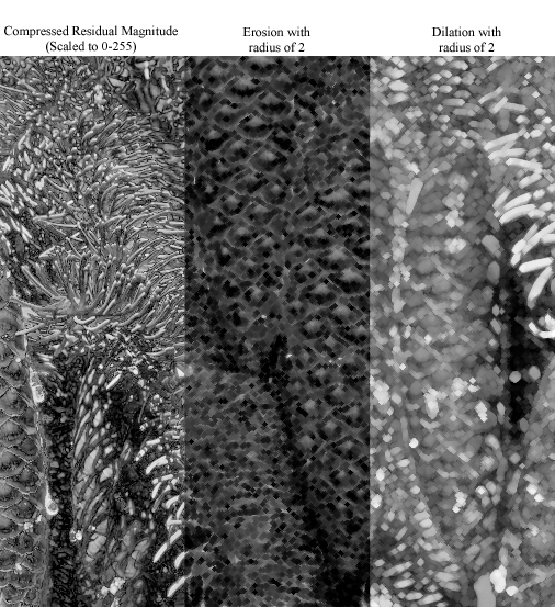
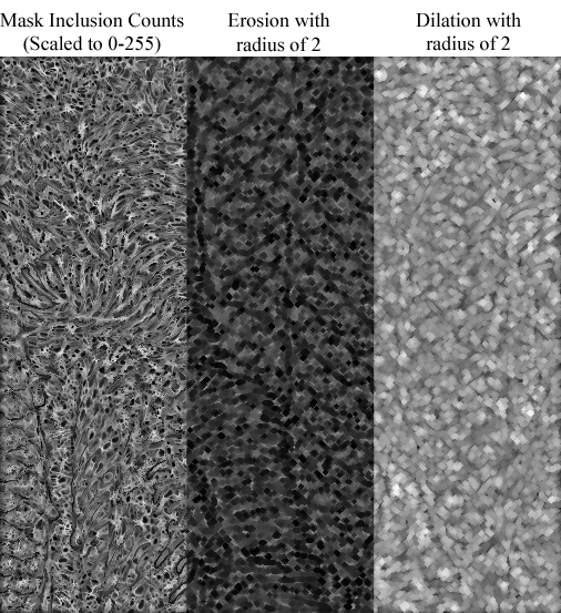
The following images are examples of weighting images produced using the methods described in the Introduction above:

Magnitude of the compressed residual, obtained at a filtering mask size of 64

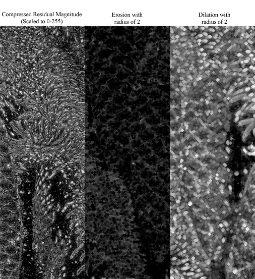
Magnitude of the compressed residual, obtained at a filtering mask size of 1024

Mask inclusion counts produced with a filtering mask size of 64

Mask inclusion counts produced with a filtering mask size of 1024

Texture Images

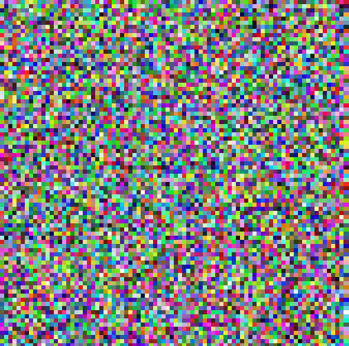
Aside from the images of mask inclusion counts shown above (they were used as weighting images and/or texture images), I used the following random checker pattern as a texture image:

Texture Addition using a Pattern of Random Checkers

All results in this section were made by preferentially re-texturing non-outlier pixels.

Weighting by the magnitude of the compressed residual, obtained at a filtering mask size of 64

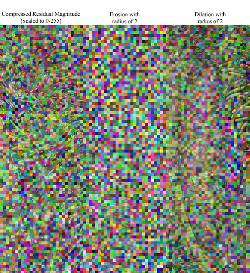
Weighting by the magnitude of the compressed residual, obtained at a filtering mask size of 1024

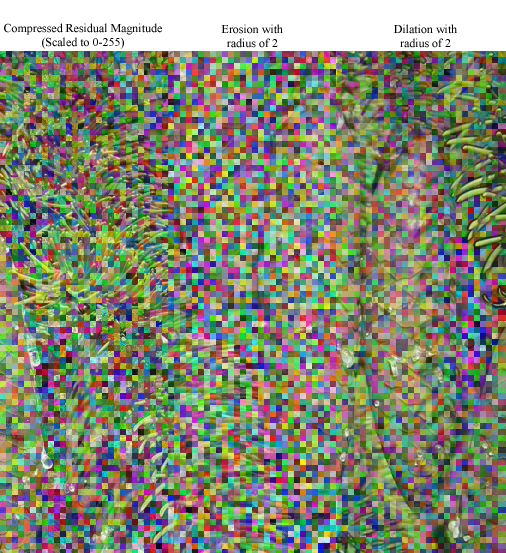
Weighting by the counts of mask inclusions obtained at a filtering mask size of 64

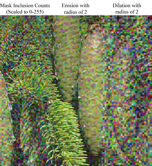
Weighting by the counts of mask inclusions obtained at a filtering mask size of 1024

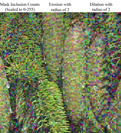
Discussion

When weighting the average by the magnitude of the compressed residual, I find that the residual obtained at a larger mask size gives nicer results, because different regions in the image have increasingly different average weightings. In contrast, when weighting by counts of mask inclusions, I prefer using mask inclusions obtained at a smaller mask size, since there is more local variation in weights, adding texture to otherwise uniformly-retextured areas.

Generally, I find that processing the weighting image by morphological erosion or dilation is undesirable, as the weighting image loses some of its texture. Furthermore, at high disk structuring element radii, edges in the source image acquire unnatural borders in the retextured image.

While not shown in this post, I also tried calculating the residual using a two-pass filtering method (as described in my last post at http://gigl.scs.carleton.ca/node/539. Using a two-pass approach was more or less equivalent to decreasing the mask size used in the single-pass approach, in that the addition of texture was less varied across the regions of the image.

Texture Addition using Mask Inclusion Counts

When weighting the addition of mask inclusion counts as texture, I tried both preferentially re-texturing outliers and non-outliers and found that it was hard to decide which method I liked. The two approaches have different effects which are not easily compared.

The results shown below were made without the use of morphological erosion or dilation on the weighting image. Furthermore, unlike the rest of this post, all weights assigned to the new texture (mask inclusion counts) were in the range 0-0.5. Based on the results of adding a random checker texture to the image shown above, I had decided that weights from 0-1 were on average too high.

Re-texturing non-outliers, weighted by counts of mask inclusions

Re-texturing outliers, weighted by counts of mask inclusions

Re-texturing non-outliers, weighted by the magnitude of the compressed residual

Re-texturing outliers, weighted by the magnitude of the compressed residual

A useful point of comparison for the above results is a simple unweighted average of the source image with the image formed by counts of mask inclusions:

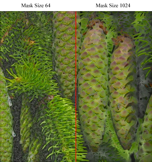
Unweighted averaging of the source image lightness channel with textures formed by mask inclusion counts

Discussion

In all cases, using mask inclusion counts obtained at a smaller mask size as a texture image gave better results with more intricate textures.

When weighting the texture addition by counts of mask inclusions, I preferred using mask inclusion counts produced at a smaller mask size, as this increased the amount of texture in the output image. However, when retexturing non-outliers more strongly, small features in the output image, such as the sap droplets on the pinecones, had slightly less contrast with the background than when I used mask count inclusions produced at a large mask size (1024 pixels). The reverse seemed to be true when retexturing outliers more strongly than non-outliers.

When weighting the texture addition by the magnitude of the compressed residual, I preferred using a residual obtained at a lower mask size when retexturing outliers, and a residual obtained at a higher mask size when retexturing non-outliers. Both of these combinations resulted in the most tonal contrast in the output image, especially between the sap droplets and the background.

Finally, comparing all other results with the unweighted average of the source image's lightness channel with the counts of mask inclusions (last image above) makes it apparent that trying to vary the amount of retexturing throughout the image is worthwhile. The unweighted average is less interesting than the weighted averages, because it is highly uniform in texture.

(Image Source: Bernard Llanos)