Introduction

The MATLAB language is ideal for writing prototype programs very quickly, as MATLAB provides a large number of built-in functions and it is possible to run code fragments without embedding them in a full program with a "main" function, header files, etc. Unfortunately, MATLAB programs are interpreted as opposed to compiled and run more slowly than compiled C programs, for example.

On the other hand, it is possible to take advantage of both the speed of C and the ease of use of MATLAB by writing MEX-functions in C. I decided to use this approach in order to obtain a faster cumulative range geodesic filtering program than the MATLAB code version which I had written earlier.

Filter Mask Generation Using a Binary Heap

Seeking to improve the speed of the cumulative range geodesic filtering program described in my last blog entry, I started by examining code for Dijkstra's algorithm written by David Gleich (downloaded from http://www.mathworks.com/matlabcentral/fileexchange/24134-gaimc-graph-algorithms-in-matlab-code ). I had been using this code to produce data with which I could compare my results to determine if my program was working correctly. David Gleich's code, which uses a binary heap, ran significantly faster than my program.

Using David Gleich's program and some general information on binary heaps as guides, I substituted the Fibonacci heap with a binary heap. The version which used a Fibonacci heap processed an image at a rate of around one pixel per second, while the version with a binary heap, following some initial changes to improve its efficiency, reached a speed of about 50 pixels per second. After working much harder on optimizing the code, the filter ran at about 350 pixels per second.

Introduction

The cumulative range geodesic image filter was first developed by Dr. Mould in 2012, and is described in the following article:

Image and Video Abstraction using Cumulative Range Geodesic Filtering, Computers & Graphics, 2013.

(Available here on this website)

This term, I will work on modifying the filter to see what results it can produce, and also to explore a few applications beyond simply stylizing images.

First, however, I am building my own version of the filter in order to become familiar with the details of the implementation.

One of the features of ths project is to let all particles grow themselves yet not crossing with each other.  Each particle is stored in array, and knows the distances with two adjecent neighbors. When two neighboring particles grow too close to each other, one of them will be killed to avoid collision. However, when two particles which are not neighbors about to cross, they cannot simply be alerted using this method.

We try to solve this with the idea below:

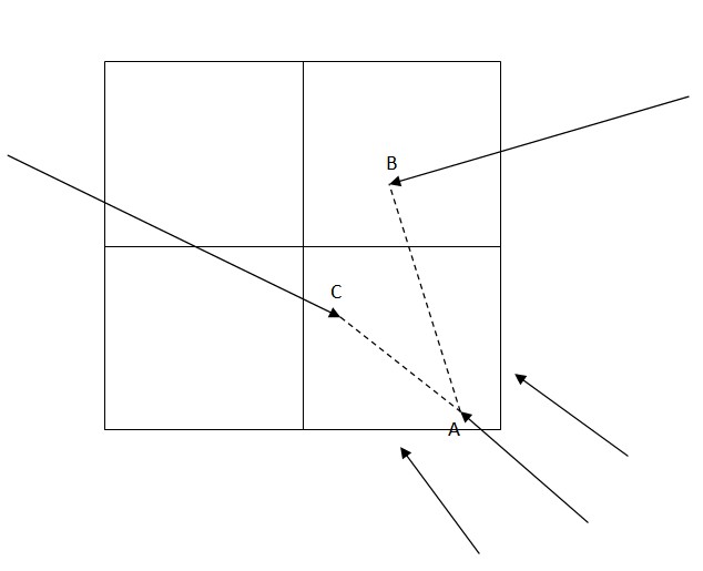
1. Divide the whole screen into grid cells, the size of the grid cells can be changed as need. Each particle will remember the grid ID that it is currently in and register in that grid. If the total number of particles that have registered in the grid cell exceeds a threshold, the grid then is blocked and no new particles could enter. When a particle enters a new grid cell, it will: a) Check if this grid cell is still available. b) If the grid is still vacancy, update its current grid ID and register in the grid.
2. There are two cases of collision: collide with particles which are also currently inside the grid; collide with the traces which are left by particles before.
3. The possible solution to prevent the cases is:  Get the information of other registered particles, check the distance with them, kill if needed; When there is a particle enter and leave without collisions, or two particles died, the grid cell is then marked as blocked, no more future particles can enter.

For example: As shown in figure below, when particle A enters this grid, it gets the information of B and C, thereby keeping checking the distance between each other. A, B and C can be killed all together when there is a death need.

I wrote a summary of this year's GRAND meeting from my perspective on my personal blog:

Last week, I attended the annual meeting of the GRAND (Graphics, Animation, and New Media) research network, held in Toronto.  Although the research and discussion presented and held at the conference spanned much more, the focus for me was on games and stories in games.

Read the whole post here.

1. Problem

As shown in the figure 1, assume there are two particles A and B moving parallel, the distance between A and B is known, and d(AC) = d(CB). Now we add a new particle V starting from A's position, moving towards the middle line of AB. Point R shows the x-coordinate of V.

This post aims the problem of defining V's movement so that the path of it will shape a smooth tangent-like curve as shown in figure 1.

        (figure 1)

2. Solution

1) Get corresponding tangent value of particle's location

First, we need to transform particle's coordinate so that we could use it in tangent function.

We know that:

Distance of A and R: d(AR)     (NOTE: In practice, since A and B move together with point V, so it should be fine to use d(AV) directly)

Distance of A and C: d(AC)

Let a float type ratio = d(AR) / d(AC). Since the path in figure 1 is one cycle in tangent function from -PI/2 to PI/2 (see figure 2 red curve), if we define X(x,y) as a corresponding point of V on tangent's graph, then: 

ratio = d(A'x) / d(A'C')   (NOTE: A' = -PI/2 and C' = PI/2, x here is the value of x-coordinate)

         = d(A'x) / PI

For each position of V on path p, we could find the corresponding tangent value as tan(x). For example:

d(A'x) = PI * ratio;

x = d(A'x) - A = PI * ratio - PI/2; 

then the corresponding tangent value of V at that time could be obtained from tan(PI * ratio - PI/2)

 (figure 2)

2) Get slope value

Apparently, the tangent line of the red curve in figure 2 gives the direction of particle V at each moment. We know that: slope value = tangent of the angle of the slope, so we need to get the slope value of tan(x) by taking derivative:

slope = d/dx * tan(x) = sec(x) * sec (x)

As shown in figure 2, the blue dash line indicates the derivative of tan(x), point S in y-coordinate is the corresponding slope value of X. 

The angle of the slope could be obtained:

angle = arctan(slope).

3) Get direction

By now, we got the angle of the slope of path p, aka, the angle of V's direction.

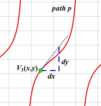
   (figure 3)

In figure 3, V1 locates at (x,y), the blue tangent line points the current direction. For each unit value dx, we could get the dy by tan(angle). So the direction of V1 could be obtained as:

dir.x = 1;

dir.y = tan(angle);

dir.normalize();         (NOTE: since tan(angle) = slope, we could also skip the step calculating angle and simply use slope)

Now we get the general method to calculate a particle's direction moving along a tangent-like path.

At anytime, simply use:

pos.x += v * dir.x;

pos.y += v * dir.y;      (NOTE: vector "pos" denotes the current postion of a particle, scalar "v" represents the speed)

to update the particle's position.

I was invited to speak at the Canadian University Software Engineering Conference in Montreal this January.  These are the slides from my talk on interactive storytelling:

I went to another conference this week and wrote about my experience on my blog:

I went to Montreal on Wednesday to present my work on what makes augmented reality good for learning (and in general, really).  The conference was the World Conference on E-Learning in Corporate, Government, Healthcare & Higher Education (or just E-Learn for short).  It was an interesting experience, but in the end, not entirely satisfying for me personally.

You can read the whole post and see my presentation slides here.

Last week, I attended the Grace Hopper Celebration of Women in Computing in Baltimore.  I wrote up a few blog posts on my personal blog about the conference:

• The Road to GHC12 is a picture-filled post about our road trip through Vermont and Connecticut on our way to Baltimore.
• Lili Cheng: Creativity, Learning, and Social Software (GHC12) is about a really cool group at Microsoft Research called FUSE Labs (they make Kodu!).
• Go Lean, Go Agile: Are We There Yet? (GHC12) is my take on the discussion about agile software development.
• NSF Funding Opportunities and Effective Proposal Writing Strategies (GHC12) offers what the title says; I also talk about how the advice relates to one of my own projects.

In just over a week, hundreds of students (mostly in grade eight) will descend upon Carleton for our annual mini-courses.  This year, a colleague and I will be doing something a little different in our course:

I've wondered in the past how important interactive storytelling might be in educational games.  The  potential to use story for more than just engagement seems high.  In just over a week, a colleague and I are going to run an experiment that will test how useful (not necessarily interactive) story is in teaching computer science concepts to complete beginners.

Read all about it on my personal blog.